[From scrying, mini-scrying and GPS.]
Simple plot over time
Where we have a single data source (for example, sampled white noise), as a long list of numbers (0-1024) like this:
374
427
442
425
428
436
454
438
443
462
443
444
464
442
454
in a file called “overnightwhitenoise”
which can be plotted using gnuplot from the command-line or from within GNU Emacs.
Commandline:
Enter at the prompt the command:
gnuplot
and then at the gnuplot prompt:
plot "overnightwhitenoise" with lines
with the file overnightwhitenoise in our current directory will show the plotted data on the screen
other commands from within gnuplot
Set commands are issued before the plot command to set parameters within gnuplot. Once set we use the command “unset” eg.
unset title
- to plot to an image file/png
set term png size 1024,768
set output "overnightwhitenoise.png"
and then the plot command. We should have the png file in our current directory
- to change current directory
cd "/root/projects/detection/logs"
- to get help on commands
help plot
- to plot only part of a data set on each axis (ie. to narrow down to a certain point in time or a range of values on the y scale)
plot [0:2000] "overnightwhitenoise" with lines
to narrow to first 2000 values on the time(x) axis
plot [0:][300:400] "overnightwhitenoise" with lines
to narrow the range from 300 to 400 only on the y axis
- labelling
for the title of the plot
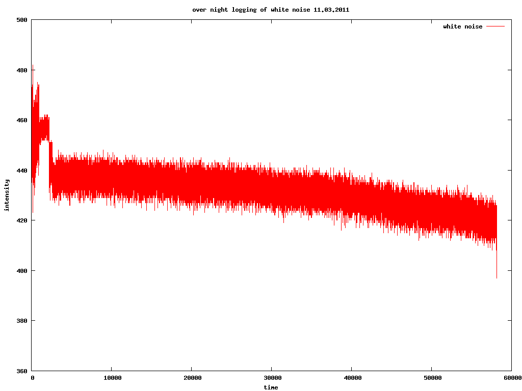
set title "over night logging of white noise 11.03.2011"
to label the axes
set xlabel "time"
set ylabel "intensity"
to label the index/data
plot "overnightwhitenoise" w lines title "white noise"
- squeezing the data by division
plot "overnightwhitenoise" using ($1/400) w lines
divides the y axis data by 400
GNU Emacs
Open a file or a buffer with gnuplot commands.
M-x gnuplot-mode
Select a region and send to/execute in gnuplot with:
C-c C-r
or
M-x gnuplot-send-region-to-gnuplot
And:
C-c C-l ;; to send a line
C-c C-b ;; to send the buffer
and in org-mode/org-babel
In the .org file we have:
#+begin_src gnuplot :file whitenoise.png
set ylabel "intensity"
set xlabel "time"
plot "/root/projects/detection/logs/overnightwhitenoise" with lines
#+end_src
The result
More advanced two dimensional plots
plotting in real time from a serial port stream
using gnuplot and minicom
We have data from the serial port being written as a series of numbers to a log file. In minicom we use
C-z l
to log to the file in real time.
We have a gnuplot script called looper which reads that file (called test2)
a=a+1
plot "/root/test2" with lines
pause 0.1
if(a<50000) reread
Opening gnuplot from the commandline we use:
a=0
load "looper"
using python, wx and matplotlib
Using code from https://github.com/gregpinero/ArduinoPlot with a few changes/additions to Arduino_Monitor.py
- to alter serial port location and arguments - to write a log of the incoming data
- Arduino_Monitor.py
"""
Listen to serial, return most recent numeric values
Lots of help from here:
http://stackoverflow.com/questions/1093598/pyserial-how-to-read-last-line-sent-from-serial-device
"""

from threading import Thread
import time, datetime
import serial


# TODO: add logging to next numerical file named here

last_received = ''
def receiving(ser):
    global last_received
    buffer = ''
    while True:
        buffer = buffer + ser.read(ser.inWaiting())
        if '\n' in buffer:
            lines = buffer.split('\n') # Guaranteed to have at least 2 entries
            last_received = lines[-2]
            #If the Arduino sends lots of empty lines, you'll lose the
            #last filled line, so you could make the above statement conditional
            #like so: if lines[-2]: last_received = lines[-2]
            buffer = lines[-1]


class SerialData(object):
    def __init__(self, init=50):

        now = datetime.datetime.now()
        numm=now.strftime("%Y%m%d%H%M")

        self.f = file("%s.results.log" %numm, 'w')
        try:
            # change for SERIAL PORT LOCATION
            self.ser = ser = serial.Serial('/dev/ttyUSB0', 9600, timeout=1)
        except serial.serialutil.SerialException:
            #no serial connection
            self.ser = None
        else:
            Thread(target=receiving, args=(self.ser,)).start()

    def next(self):
        if not self.ser:
            return 100 #return anything so we can test when Arduino isn't connected
        #return a float value or try a few times until we get one
        for i in range(40):
            raw_line = last_received
            try:
                self.f.write("%s\n" %raw_line.strip())
                self.f.flush()
                return float(raw_line.strip())
            except ValueError:
                print 'bogus data',raw_line
                time.sleep(.005)
        return 0.
    def __del__(self):
        self.f.close()
        if self.ser:
            self.ser.close()

if __name__=='__main__':
    s = SerialData()
    for i in range(500):
        time.sleep(.015)
        print s.next()
two plots overlayed
plot "allovernight" using ($1/400) w lines title "magnetic", "allovernight" using ($2/5) w lines title "light", "allovernight" w lines using 3 title "temp"
Scrying.mini-scry data with GPS
format of the data
From both scry and mini-scry (with GPS attached) we have data which looks like this:
5232.07020,01325.0273,256,74,3
5232.06730,01325.0736,239,51,1
5232.06710,01325.0737,259,57,2
5232.07030,01325.0778,303,82,0
As: Latitude (NMEA WGS-84), Longitude, and, in this case, intensity of high frequency signals, low frequency, 2.4GHz
(With GSR and temperature sensor attached we have: Lat, Long, high frequency, GSR and temperature).
To plot these we need to convert NMEA to decimal using the example: 5232.0702) = 52+(32.0702/60) and convert from spherical to cartesian co-ordinates.
using python and gnuplot
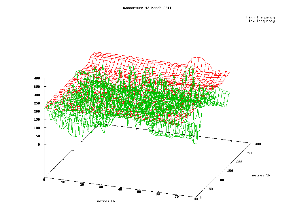
We can convert to decimal, then to cartesian, then plot these using gnuplot-pythin binding. Here's an example script for high and low frequency plot:
- gpsprocess.py
from pylab import *
import csv, os, Gnuplot, Gnuplot.funcutils

g = Gnuplot.Gnuplot(debug=1)
NMI = 1852.0
D2R = pi/180.0

def read_csv_file(filename):
    data = []
    for row in csv.reader(open(filename)):
        data.append(row)
    return data

def process_gps_data(data):
    latitude    = []
    longitude   = []
    intensity   = []
    intensitylow   = []

    for row in data:
        latitude.append(float(row[0][0:2]) + \
                            float(row[0][2:])/60.0)
        longitude.append((float(row[1][0:3]) + \
                              float(row[1][3:])/60.0))
        intensity.append(float(row[2]))
        intensitylow.append(float(row[3]))

    return (array(latitude), array(longitude), \
                array(intensity), array(intensitylow))


y=read_csv_file('/root/projects/detection/logs/scryturmcut')
(lat, long, intensity,intensitylow) = process_gps_data(y)
# translate spherical coordinates to Cartesian
py = (lat-min(lat))*NMI*60.0
px = (long-min(long))*NMI*60.0*cos(D2R*lat)
#intensitylow=intensitylow*4
newy=[]
for x,yz,z,zz in zip(px,py,intensity,intensitylow):
    newy.append((x,yz,z,zz))

#gnuplot commands
g('set parametric')
g('set style data line')
g('set surface')
g('set key')
g('unset contour')
g('set dgrid3d 40,40,10')
g('set xlabel "metres EW"')
g('set ylabel "metres SN"')
g('set label "signal intensity"at -60,0,0')
g('set view 60,20')
g.title("wasserturm 13 March 2011")
g('set term png size 1024,768')
#g('set term png size 14043,9933') # A0
g('set output "/root/projects/detection/logimages/scryturmcut.png"')

g.splot(Gnuplot.Data(newy, using=(1,2,3), with='lines', title='high frequency'),Gnuplot.Data(newy, using=(1,2,4), with='lines', title='low frequency'))
Obviously changing any parameters such as input data file and output filename.
The result is:
generating a gpx file
- In two steps using an Emacs script and gpsbabel as follows:
Emacs Lisp to convert from scrying logfile (stripped down NMEA) to decimal (fixed 15.03.2011):
- nmeatodec.el
(defun nmeatodec()
  (interactive)
  (goto-char (point-min))
  (while
      (re-search-forward "^[0-9]" nil t)
    ;; find lat, insert dec point, divide 60, insert
    (forward-char 1)
    (insert ".")
    ;; remove next .
    (re-search-forward "\\." nil t)
    (delete-char -1)
    ;; grab region and /60.
    (setq pnt (- (point) 2))
    (re-search-forward "," nil t)
    (setq decstring (buffer-substring pnt (- (match-end 0) 1)))
    (setq dec (/ (string-to-number decstring) 60))
    ;; kill and insert
    (kill-region pnt (- (match-end 0) 1))
    (goto-char pnt)
    (insert (number-to-string dec))
    (re-search-forward "," nil t)
    (forward-char 3)
    (insert ".")
    ;; remove next .
    (re-search-forward "\\." nil t)
    (delete-char -1)
    ;; same again
    (setq pnt (- (point) 2))
    (re-search-forward "," nil t)
    (setq decstring (buffer-substring pnt (- (match-end 0) 1)))
    (setq dec (/ (string-to-number decstring) 60.0)) ;; now get rid of .
        (kill-region pnt (- (match-end 0) 1))
    (goto-char pnt)
    (insert (number-to-string dec))
    (re-search-backward "\\." nil t)
    (delete-char 1)
    (forward-line 1)
    (beginning-of-line)))
We just run
M-x nmeaodec
with the logfile in the buffer, re-save as “testlog” and then run:
gpsbabel -t -i unicsv -f testlog -o gpx -F testlog.gpx
- or use the conversion utility at:
http://www.gpsvisualizer.com/convert_input
- but we need first to add this to the first line of our log file:
lat,long,elevation
using google maps/ google earth
- Convert logfile to kml for use in google earth.
gpsbabel -t -i unicsv -f testlog -o kml -F test.kml
- Use the gpsvisualizer utility to convert to kml.
http://www.gpsvisualizer.com/convert_input
(again see above for the added logfile line)
- Use the gpsvisualizer utility to overlay onto google maps.
http://www.gpsvisualizer.com/map_input?form=google
(again see above for the added logfile line)
- Upload the kml file to a server and load on google maps
using viking to overlay onto openstreetmaps
Open viking.
Select Layers (top level menu), new Map Layer (dropdown), Openstreetmaps(Osmarender).
Open the test.gpx file using File, Open.
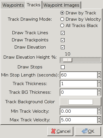
Right click on the left hand text.gpx in Layer Name frame and select Properties. Here we can select Tracks and click Draw Elevation as follows:
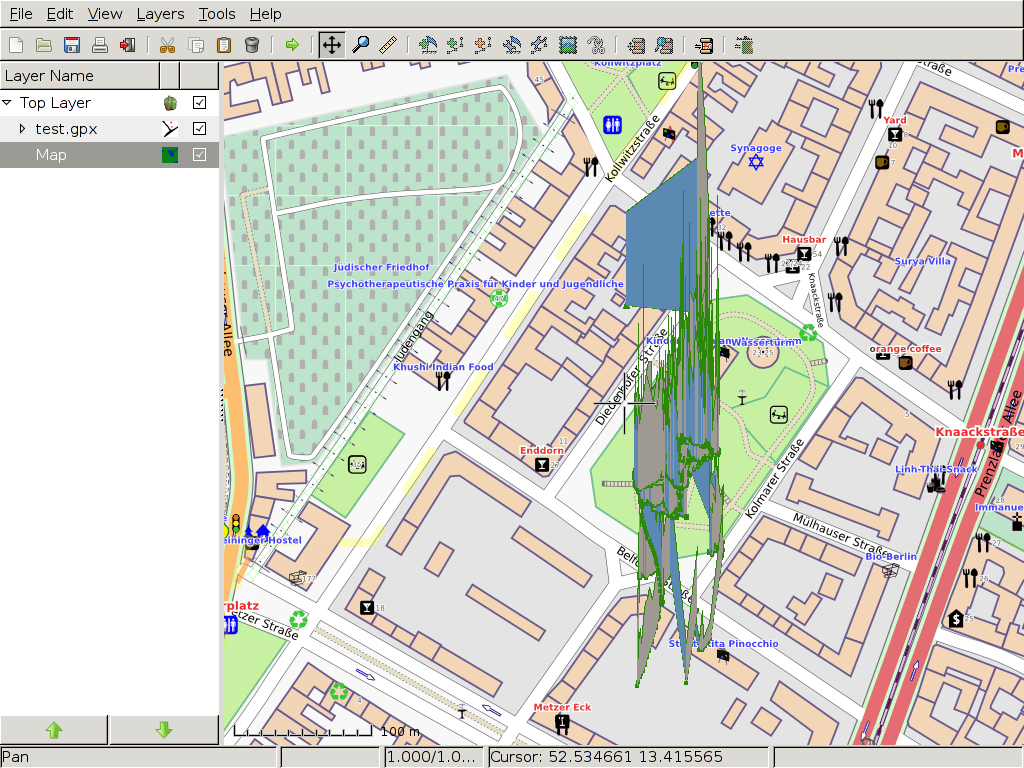
We have to move the map to see the effect.
Right click Map from the same Layer Name frame and select Download Onscreen Maps.
The Viking screen should look something like this:
more on gnuplot
- line style 3d plot:
unset view map
set ticslevel 0
set surface
unset contour
unset pm3d
unset dgrid3d
splot "/root/projects/sommercamp/120801scry.log.clean" with lines
entropy plot/location scripts
- gpsrng2.py
from pylab import *
import csv, os, Gnuplot, Gnuplot.funcutils

g = Gnuplot.Gnuplot(debug=1)

NMI = 1852.0
D2R = pi/180.0

#data = sys.argv[1]
#title = sys.argv[2]

def read_csv_file(filename):
    data = []
    for row in csv.reader(open(filename)):
        data.append(row)
    return data

def process_gps_data(data):
    latitude    = []
    longitude   = []
    intensity   = []
    lf          = []
    gsr         = []
    temp        = []
    for row in data:
        latitude.append(float(row[0][0:2]) + \
                            float(row[0][2:])/60.0)
        longitude.append((float(row[1][0:3]) + \
                              float(row[1][3:])/60.0))
        intensity.append(float(row[2]))
#        lf.append(float(row[3]))

    return (array(latitude), array(longitude), \
                array(intensity)#, array(lf))

y=read_csv_file('/root/collect2012-3/monkx')
(lat, long, intensity) = process_gps_data(y)

# what is lat, long for min/max intensity?

minty=min(intensity)
maxxy=max(intensity)

for index, item in enumerate(intensity):
    if item==minty:
        lower=index
    if item==maxxy:
        max=index

print "low entropy sites -: ",
print lat[lower], long[lower]
print "\nlow entropy sites +: ",
print lat[max], long[max]
- gpsrngcum.py
from pylab import *
import csv, os, Gnuplot, Gnuplot.funcutils

g = Gnuplot.Gnuplot(debug=1)

NMI = 1852.0
D2R = pi/180.0

#data = sys.argv[1]
#title = sys.argv[2]

def calc_limit_high_005(range):
        var = (1.96 / 2) * math.sqrt(range)
        limit_high = range/2 + var
        return limit_high

def read_csv_file(filename):
    data = []
    for row in csv.reader(open(filename)):
        data.append(row)
    return data

def process_gps_data(data):
    latitude    = []
    longitude   = []
    RNG          = []
    ppp         = []
    cnt=1
    rngcum=0
    for row in data:
        latitude.append(float(row[0][0:2]) + \
                            float(row[0][2:])/60.0)
        longitude.append((float(row[1][0:3]) + \
                              float(row[1][3:])/60.0))
        rngcum+=(100-float(row[2]))
        RNG.append(rngcum)
        ppp.append((calc_limit_high_005(cnt*200))-(cnt*100))
        cnt+=1

    return (array(latitude), array(longitude), \
                array(RNG),array(ppp))

y=read_csv_file('/root/collect2011/psych/studies/symptoms_newcastle/logs/dayoneRNG')
(lat, long, RNG, ppp) = process_gps_data(y)
# translate spherical coordinates to Cartesian
py = (lat-min(lat))*NMI*60.0
px = (long-min(long))*NMI*60.0*cos(D2R*lat)
#newintensity=intensity-min(intensity)

#pack px, py, intensity and gsr into newy
newy=[]
cummd=0
for x,yz,zz,pppp in zip(px,py,RNG,ppp):
    newy.append((x,yz,zz,pppp))

g('set parametric')
g('set style data line')
g('set surface')
g('unset key')
g('unset contour')
#g('set dgrid3d 80,80,30')
g('set dgrid3d 80,80,30')
g('set xlabel "metres WE"')
g('set ylabel "metres NS"')
#g('set label "signal intensity" at -100,0,100')
g('set view 60,20')
g.title("9th September 2011 Newcastle symptoms cumulative RNG")
#g('set term png size 14043,9933') # A0
g('set term png size 1024,768') # example
g('set output "/root/collect2011/psych/studies/symptoms_newcastle/logimages/newcumRNG.png"')
g('set style lines 1')

g.splot(Gnuplot.Data(newy, using=(1,2,3)),Gnuplot.Data(newy, using=(1,2,4)))

#g.splot(Gnuplot.Data(newy, using=(1,2,3), with='lines'))
other tricks
convert from list of values (1-1024) to a WAV file (list of numbers to audio):
in octave (start from commandline or GNU Emacs)
xx=load("overnightwhitenoise");
xxx=xx/1024
wavwrite("sound.wav",xxx)
Then open the file in audacity and - Effect → Normalize → remove DC offset and normalize amplitiude to -2.0dB
convert from WAV file to list of values for plotting
From the commandline:
sox test.wav -r 44100 -1 -u -b -c 1 test.dat
grep -v '^;' test.dat > test.datclean
and in gnuplot:
plot 'test.datclean' with lines every 1000
raw files in octave
myfile = fopen("testrnd_delay_none", "r+")
x =fread(myfile, "uchar");
hist(x)
hist(x(1:50))
plot(x)
fclose(myfile)
using viking to edit waypoints (from GPS only)
1] Acquire GPS works for Garmin (/dev/ttyUSB0)
2] Once acquired expand the Acquired left item and waypoints. Right click on an expanded waypoint and select GOTO
3] Maps - Add new map layer. Openstreetmap seems to work best. Make sure is moved down below our gps layer. Right click always to change options.
4] Crtl - + for zoom out and in.
5] Make a new TrackWayPoint layer and cut and paste tracks or waypoints into this and then right click to export this layer.
Viking reference: http://viking.sourceforge.net/mediawiki/index.php/Viking\_Reference\_Manual#Export
using viking to edit tracks
- zoom in until we can see trackpoints
- click on icon from icon bar to select edit trackpoints
- clikc on trackpoint and edit dialogue opens with:
using gpsman to select track from GPS
can't run as root: remember on root: xhost +)
extract one gps track from gpx:
1] open in gpsman (running as xxxxx)
2] import gpx
3] go to data/track/export/gpx/select
using gpsman to edit scrying tracks
1] import GPX file
2] go to items (bottom panel) → display on map → tracks
3] double click on track and delete/edit
using gpsbabel to download files from garmin device
gpsbabel -t -i garmin -f /dev/ttyUSB0 -o gpx -F gpsfile.gpx
links
gpsman working with tracks: http://www.words2u.net/pmwiki/?n=GPSMAN.9WorkingWithTracksBasicOperations
NMEA to decimal and googlemaps view: http://www.hiddenvision.co.uk/ez/


